Making of a Deep Learning Framework - Part 1
Recently, I was implementing a neural network from scratch and it got me thinking about “what goes on under the hood of a deep learning framework?” Having used Pytorch for quite some time now, I have always treated everything like a magic trick - I am happy with what I see (the results!), but I don’t know what is going on! Subsequently, this got me into reading some brilliant blog posts and books on how to implement a deep learning framework.
The core of any deep learning framework is its ability to auto differentiate any function through backpropagation, no matter how complex it is. Although the concept is not rocket science and is relatively easy to understand when trying to derive it on paper, this is only the case (for me, at least) for univariate examples. Any attempt trying to derive a general vectorized formula for the procedure quickly becomes messy and untractable.
Having struggled for quite some time, I thought I should go ahead and implement it with whatever knowledge I have now and just fill in the gaps as I go along. Perhaps, through implementing it, something will click in my brain, and I will finally be able to understand it! Before we dive into the coding part, I think it is useful to briefly go over the auto differentiation algorithm, (aka backpropagation).
Note, at the time of writing the first part, my foresight tells me that this iteration of my deep learning framework will be extremely inefficient as I am aiming to dive deep into the mechanisms and thus will probably not utilise numpy efficient vectorised operations, i.e. I will use a lot of for loops (I think). However, as I gain a better understanding of the implementation, I hope future iterations will be more efficient
Backpropagtion
For a function $f(x)$, the derivative of $f$ w.r.t $x$ is denoted by $f’(x)$, or $\frac{df}{dx}$.
For a chained function of $x$, e.g. $f(g(x))$, the derivative of f w.r.t x is denoted by $f’(x)g(x) + g’(x)f(x)$, or
\(\frac{df}{dx} = \frac{df}{df}\frac{df}{dz} \frac{dz}{dx}\) where $z = g(x)$
Going further, for $f_N(f_{N-1}(\dots (f_1(x)))$, the derivative of the output w.r.t $x$ is \(\frac{df_{N-1}}{dx} = \frac{df_N}{df_N}\frac{df_{N}}{dz_{N-1}}\frac{dz_{N-1}}{dz_{N-2}}\dots\frac{dz_1}{dx}\) where $z_i = f_i(x) \forall i \in {2,3, \dots , N-1}$
In the above, we denoted the intermediate functions with $z_i$ instead of using $f$ because I think it makes it easier to differentiate between the final output function/value, and the intermediate values.
Furthermore, note that we have included the term \(\frac{df}{df} = 1\) because it will be useful later on, so bear with me here (:)).
All in all, the above equations are just for formalaity and in fact, I find those lines of equations to be rather confusing and doesn’t properly capture the inner mechanics of what backpropagtion is actually doing (they are useful if you are doing maths though…). Therefore, let’s go through an example:
- $z_1 = f_1(x) = 2x$
- $ z_2 = f_2(f_1(x)) = (2x)^2 = 4x^2$, or simply $f_2(z_1) = z_1^2$,
- $f_3(f_2(f_1(x))) = cos[(2x)^2]$, or simply $f_3(z_2)=cos(z_2)$
I hope you have noticed the pattern after the example above, if not let me try to explain it. Note that each layer, in the reversing order is just the derivate of the current layer multiplied by the past layer, more concretely, we start from the last layer and approach towards the layer we want the derivative for:
- $N = 3$, $f_3(z_2) = cos(z_2) \implies f’(z_2) = -sin(z_2)$
- $N = 2$, $f_2(z_1) = z_1^2 \implies f’(z_1) = 2z_1$
- $N = 1$, $f_1(x) = 2x \implies f’(x) = 2$
multiplying each layer’s derivatice “output”, the result is \(-sin(z_2) \cdot 2z_1 \cdot 2 = -sin(2x^2) \cdot 4x \cdot 2 = -8xsin(2x^2)\)
One thing that I overlooked when I was doing my reading up was forgetting that “$x$”, the input is always known, e.g. think of $x$ as the parameter we are tuning, such that \(f(x_{t+1}) < f(x_t)\) We always know exactly what value it is, as we always have a “guess”. Therfore, for each of the derivative $-sin(z_2)$, $2z_1$, and $2$, we know their exact value (at the current iteration) and all we need to do to calculate the gradient is to “cache” the “local” gradient w.r.t each intermediate parameter.
Now, let’s make it more even more concrete by setting $x = 2$, i.e. we are trying to find the derivative of \(y = cos((2x)^2)\) at x = 2.
Note, before we used $f_i$ to demonstrate the layer nature of the function, but now let’s denote $y$ to be the final output, i.e. \(y = f_3(z_2) = f_3(f_2(z_1)) = f_3(f_2(f_1(x)))\) (we don’t use $z_3$ because we want to ditinguish between an intermediate funciton output $z_i$, and the final output $y$)
The algorithm is split into two parts, the forward pass, and the backward pass (backpropgation). During the forward pass, each layer is calculated, e.g.
Forward Pass
-
we get $z_1 = 2(2) = 4$, we also calculate the “local” gradient of the function here w.r.t x, e.g. $\frac{dz_1}{dx} = 2$ and store it in as a attribute to the input “x.grad = 2”, say.
-
We then go to the second layer z_2 = $z_1^2$, we know what $z_1 = 4$ is so we know the local gradient is $\frac{dz_2}{dz_1} = 2z_1 = 2(4) = 8$ and store it in “z_1.grad = 8”, say.
-
Finally, we work out $y = cos(z_2) = cos(8)$ and its local gradient $\frac{dy}{dz_2} = -sin(8)$ and store it at “z_2.grad”, say.
Backward Pass As the name suggests, we work backwards for this part
-
Up until now, we have not mentioned the local gradient of y yet. This is just $\frac{dy}{dy} = 1$
-
Trace the operation before obtaining y, which is cos(z_2), with local gradient $\frac{dy}{dz_2} = -sin(8)$, we get \(\frac{dy}{dy}\frac{dy}{dz_2} = (1)\cdot(-sin(8))\)
-
Trace the operation before $z_2$, which is $z_2 = 2z_1$ with local gradient 8, we get \(\frac{dy}{dy}\frac{dy}{dz_2}\frac{dz_2}{dz_1} = (1)\cdot(-sin(8))\cdot(8)\)
-
Trace the operation before z_1, whcih is $z_1 = 2x$ with local gradient 2, we get \(\frac{dy}{dy}\frac{dy}{dz_2}\frac{dz_2}{dz_1}\frac{dz_1}{dx}= \frac{dy}{dx} = (1)\cdot(-sin(8))\cdot(8)\cdot(2) = -16sin(8)\) which matches with the analyical solution we obtained above.
A custom class
For our autograd system, we will work with scalar values. The built in python object classes such as int, float, double should suffice, but will make the code rather cumbersome and inconvenient. Thus, to simplify for our downstream task (working out the gradient), we shall create a custom class that stores the scalar number as well as some other metadata useful for our task. This class should be able to return its gradient with respect to the series of mathematical operations carried out on it, e.g. for \(y = cos((2x)^2)\) we should be able to obtain the gradient \(\frac{dy}{dx}\) with a simple call such as “$x$.grad”.
For this reasom, we make the following custom class “Scalar”:
import numpy as np

class Scalar:
    def __init__(self, num):
        self.num = num
        self.grad = 0
        self.creators = None

    def backward(self):
        if self.creators is not None:
            for c in self.creators:
                c.grad *= self.grad
                c.backward()

    def __mul__(self, other):
        x = self.num
        z = other.num
        y = Scalar(x * z)
        y.creators = [self, other]
        dy_dx = z
        dy_dz = x
        self.grad += dy_dx
        other.grad += dy_dz

        return y

    def __add__(self, other):
        x = self.num
        z = other.num
        y = Scalar(x + z)
        y.creators = [self, other]
        dy_dx = dy_dz = 1
        self.grad += dy_dx
        other.grad += dy_dz

        return y

    def __sub__(self, other):
        x = self.num
        z = other.num
        y = Scalar(x - z)
        y.creators = [self, other]
        dy_dx = 1
        dy_dz = -1
        self.grad += dy_dx
        other.grad += dy_dz

        return y

    def __truediv__(self, other):
        x = self.num
        z = other.num
        y = Scalar(x / z)
        y.creators = [self, other]
        dy_dx = 1 / z
        dy_dz = -1 / z**2
        self.grad += dy_dx
        other.grad += dy_dz

        return y

    def __pow__(self, power, modulo=None):
        x = self.num
        y = Scalar(x ** power)
        y.creators = [self]
        dy_dx = power * x
        self.grad += dy_dx

        return y
The method
        def __init__(self, num):
            self.num = num
            self.grad = 0
            self.creators = None
initiliazes our “Scalar” class with 3 attributes.
- Its value (num),
- Its local gradient (grad; default to 0, or sometimes None by other people) to store the local gradients on the operations acted on it.
- Its creators, which is required to trace back a number’s root for the backpropgation to work. For our example above, $y$ would have creator $z_2$, $z_2$ would have creator $z_1$, and $z_1$ would have creator $x$
The method
        def backward(self):
            if self.creators is not None:
                for c in self.creators:
                    c.grad *= self.grad
                    c.backward()
is called when we want to work out the gradient of every scalar value involved in a particular expression. Note the first line means the calculation stops when we reach a scalar with creators as None, e.g. $x$ from our example.
The magic methods such as
        def __mul__(self, other):
            x = self.num
            z = other.num
            y = Scalar(x * z)
            y.creators = [self, other]
            dy_dx = z
            dy_dz = x
            self.grad += dy_dx
            other.grad += dy_dz

            return y
are invoked when we use the multiplcation “*” (or + for __add__, etc) operation on two “Scalar” class objects, e.g.
        Scalar(2) + Scalar(3) = Scalar(5)     -> __add__
        Scalar(2) * Scalar(3) = Scalar(5)     -> __mul__
        Scalar(2) / Scalar(3) = Scalar(3/5)   -> __truediv__
        Scalar(2) - Scalar(3) = Scalar(2 - 3) -> __neg__
        Scalar(2)**p = Scalar(2**p)           -> __pow__
Different to a regular $x$ “*” $z$ operation on python’s int or float class, which only returns the resulting value, we also creat a new “Scalar” object which carries the resulting number, as well as the metadata required for backpropagation, and also updates the local gradients for parent objects, in our case the “creators” of $y$.
Note, the way we have defined our “Scalar” class makes it work even for multivariate functions, that is one thing off the list we should worry about!
Function Differentiaion Experiments
To see how this works, we will demonstrate with the following examples”
- \[y = x^2 \text{for} x = 3\]
- \[y = x + z - u^2 \text{ for } x = 3, z = 2 \text{ and } u = 6\]
- \[y = x * z \text{ for } x = 3 \text{ and } z = 2\]
print("Example 1. y = x^2 at x = 3")
x = Scalar(3)
y = x**2
y.grad = 1 # this step is required because its value is defaulted to 0, and dy/dy = 1
y.backward() # backprop.
print("dy/dx =",x.grad) # we should get 2 * x, which is 6 in our case as x = 3


print("\nExample 2. y = x + z - u^2 at x = 3, z = 3, and u = 6")
x, z, u = Scalar(3), Scalar(2), Scalar(6)
y = x + z - (u**2)
y.grad = 1
y.backward() # backprop.
print("dy/dx =",x.grad) # we should get 1
print("dy/dz =",z.grad) # we should get 1
print("dy/du =",u.grad) # we should get -12

print("\nExample 3. y = x * z at x = 3, and z = 2")
x, z = Scalar(3), Scalar(2)
y = x * z
y.grad = 1
y.backward()
print("dy/dx =", x.grad) # we should get 2
print("dy/dz =", z.grad) # we should get 3
Example 1. y = x^2 at x = 3
dy/dx = 6

Example 2. y = x + z - u^2 at x = 3, z = 3, and u = 6
dy/dx = 1
dy/dz = 1
dy/du = -12

Example 3. y = x * z at x = 3, and z = 2
dy/dx = 2
dy/dz = 3
To work out the gradient for more complex functions, we simply follow a similar structure as how we have written the operations magic methods for the “Scalar” class. For simplicity, we only wrote 3 functions here:
def exp(input):
    x = input.num
    y = Scalar(np.exp(x))
    dy_dx = np.exp(x)
    input.grad += dy_dx
    y.creators = [input]
    return y

def square(input):
    x = input.num
    y = Scalar(x ** 2)
    dy_dx = 2 * x
    input.grad += dy_dx
    y.creators = [input]
    return y

def cos(input):
    x = input.num
    y = Scalar(np.cos(x))
    dy_dx = -np.sin(x)
    input.grad += dy_dx
    y.creators = [input]
    return y
To test out implementation, we will test the gradient we obtain with the result from calculating the finite diffierence of the function, i.e. for a small value h \begin{equation} \text{$x$.grad} \approx \frac{f(x + h) - f(x - h)}{2h} \end{equation}
print("1. y = exp(x) for x = 3, h = 0.0001")
x = Scalar(3)
y = exp(x)
y.grad = 1
y.backward()
print(f"Backprop. {x.grad:.4f} vs finite dif. {(np.exp(3 + 0.0001) - np.exp(3 - 0.0001)) / (2 * 0.0001):.4f}")

print("\n2. y = x^2 for x. = 3, h = 0.0001")
x = Scalar(3)
y = square(x)
y.grad = 1
y.backward()
print(f"Backprop. {x.grad:.4f} vs finite dif. {(np.power(3 + 0.0001, 2) - np.power(3 - 0.0001, 2)) / (2 * 0.0001):.4f}")

print("\n3. y = cos(x) for x. = 3, h = 0.0001")
x = Scalar(3)
y = cos(x)
y.grad = 1
y.backward()
print(f"Backprop. {x.grad:.4f} vs finite dif. {(np.cos(3 + 0.0001) - np.cos(3 - 0.0001)) / (2 * 0.0001):.4f}")
1. y = exp(x) for x = 3, h = 0.0001
Backprop. 20.0855 vs finite dif. 20.0855

2. y = x^2 for x. = 3, h = 0.0001
Backprop. 6.0000 vs finite dif. 6.0000

3. y = cos(x) for x. = 3, h = 0.0001
Backprop. -0.1411 vs finite dif. -0.1411
Now, lets try for more complex equations
print("1. y = exp((x+z)^2), at x = 3, z = 2, and h = 0.0001")
x = Scalar(3)
z = Scalar(2)
y = exp(square(x+z))
y.grad = 1
y.backward()
f = lambda x, z, h: np.exp(np.power(x+z+h, 2))
print(f"dy/dx\nBackprop. {x.grad:.4f} vs finite dif. {(f(3, 2, 0.0001) - f(3, 2,-0.0001)) / (2 * 0.0001):.4f}")


print("\n2. y = u*exp((x+z)^2), at x = 3, z = 2, u = 6 and h = 0.0001")
x = Scalar(3)
z = Scalar(2)
u = Scalar(6)
y = u * exp((x+z)**2)
y.grad = 1
y.backward()
f = lambda x, z,u, h, h_u: (u + h_u)*np.exp(np.power(x+z+h, 2))
print(f"dy/dx\n Backprop. {x.grad:.4f} vs finite dif. {(f(3, 2, 6, 0.0001, 0) - f(3, 2, 6, -0.0001,0)) / (2 * 0.0001):.4f}")
print(f"dy/du\n Backprop. {u.grad:.4f} vs finite dif. {(f(3, 2, 6, 0.0, 0.0001) - f(3, 2, 6, 0,-0.0001)) / (2 * 0.0001):.4f}")

print('\n3. y = cos(exp(cos(x^2))) at x = 3')
x = Scalar(3)
y = cos(exp(cos(square(x))))
y.grad = 1
y.backward()
f = lambda x, h: np.cos(np.exp(np.cos((x+h)**2)))
print(f"dy/dx\n Backprop. {x.grad:.4f} vs finite dif. {(f(3, 0.0001) - f(3, -0.0001)) / (2 * 0.0001):.4f}")


print('\n3. y = cos(exp z * (cos(x^2))) at x = 3, z = 2, and h = 0.0001')
x = Scalar(3)
z = Scalar(2)
y = cos(exp(z * cos(x**2)))
y.grad = 1
y.backward()
f = lambda x, z, h_x, h_z: np.cos( np.exp((z + h_z) * np.cos((x+h_x)**2)))
print(f"dy/dx\n Backprop. {x.grad:.4f} vs finite dif. {(f(3, 2, 0.0001, 0) - f(3, 2, -0.0001, 0)) / (2 * 0.0001):.4f}")
print(f"dy/dz Backprop. {z.grad:.4f} vs finite dif. {(f(3, 2, 0, 0.0001) - f(3, 2, 0, -0.0001)) / (2 * 0.0001):.4f}")
1. y = exp((x+z)^2), at x = 3, z = 2, and h = 0.0001
dy/dx
Backprop. 720048993373.8588 vs finite dif. 720049120580.8258

2. y = u*exp((x+z)^2), at x = 3, z = 2, u = 6 and h = 0.0001
dy/dx
 Backprop. 4320293960243.1533 vs finite dif. 4320294723485.1074
dy/du
 Backprop. 72004899337.3859 vs finite dif. 72004899337.4634

3. y = cos(exp(cos(x^2))) at x = 3
dy/dx
 Backprop. 0.3891 vs finite dif. 0.3891

3. y = cos(exp z * (cos(x^2))) at x = 3, z = 2, and h = 0.0001
dy/dx
 Backprop. 0.1287 vs finite dif. 0.1287
dy/dz Backprop. 0.0237 vs finite dif. 0.0237
Machine Learning Experiements
Through the series of experiments above, we may assume that our system is working as intended. Now, let us extend our experiments to a machine learning context, i.e. using gradient descent to recover the weights from some initialisation:
- Linear regression - $y = b + x_1w_1 + \epsilon$
- Linear Regression - $y = b + x_1w_1 + x_1^3w_x\epsilon$
- Logistic Regression - $y = \sigma(b + x_1w_1)$
def LR_data(b, w1, n = 100, noise = True):
    x1 = np.linspace(-10, 10, n)
    X = []
    y = []
    for i in range(n):
        X.append([
                  Scalar(x1[i]),
                  ])

        target = b + (x1[i] * w1)
        target += np.random.rand() if noise else 0

        y.append(Scalar(target))

    return X, y


actual_b = 2
actual_w = 5
X, y = LR_data(actual_b, actual_w, 200, True) # generate a data set with bias 2, w1 = 6 and w2 = 4

# the goal is to use grad descent to find approximations for b, w1, w2 close to their actual values
bias, w1 = Scalar(1), Scalar(1)# we initialise out model parameters to 0

for i in range(20): # we train for 10 epochs
    for j in range(len(X)): # loop through each datapoint
        x1 = X[j][0]
        target = y[j]
        y_hat = bias + (w1 * x1) # prediction with the current weight
        loss = square(target - y_hat) # calculate the loss
        loss.grad = 1 # reset the loss gradient
        loss.backward() # backpropagate the gradients, starting from loss
        # take a step towards minimum
        bias.num -= 0.001 * bias.grad
        w1.num -= 0.001 * w1.grad
        # reset everything
        bias.grad = 0
        w1.grad = 0

        x1.grad = 0
        target.grad = 0
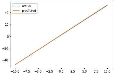
print("1. Linear Regression: y = 2 + wx + eps")
print(f"predicted bias: {bias.num:.2f}, predicte weight: {w1.num:.2f}")
print(f"actual bias: {actual_b}, actual weight: {actual_w}")

x = np.linspace(-10, 10, 100)
y1 = 2 + (5 * x)
y2 = bias.num + (w1.num * x)
print(f"Loss: {((y1 - y2)**2).mean()}")
1. Linear Regression: y = 2 + wx + eps
predicted bias: 2.51, predicte weight: 5.02
actual bias: 2, actual weight: 5
Loss: 0.2769450245415883
Plotting the resulting curve and the actual curve:
plt.plot(x, y1, label = "actual")
plt.plot(x, y2, label = "predicted")
plt.legend()
<matplotlib.legend.Legend at 0x7fda09b0b790>
def LR_data(b, w1, w2, n = 100, noise = True):
    x1 = np.linspace(-5, 5, n)
    X = []
    y = []
    for i in range(n):
        X.append([
                  Scalar(x1[i]),
                  Scalar(x1[i] ** 3)
                  ])

        target = b + (x1[i] * w1) + (w2 * x1[i]**3)
        target += np.random.rand() if noise else 0
        y.append(Scalar(target))

    return X, y


actual_b = 2
actual_w1 = 5
actual_w2 = 3
X, y = LR_data(actual_b, actual_w1, actual_w2, 30, False) # generate a data set with bias 2, w1 = 6 and w2 = 4

# the goal is to use grad descent to find approximations for b, w1, w2 close to their actual values
bias, w1, w2 = Scalar(1), Scalar(1), Scalar(1) # we initialise out model parameters to 0

for i in range(20): # we train for 10 epochs
    for j in range(len(X)): # loop through each datapoint
        x1, x2 = X[j]
        target = y[j]
        y_hat = bias + (w1 * x1) + (w2 * x2) # prediction with the current weight

        loss = square(target - y_hat) # calculate the loss
        loss.grad = 1 # reset the loss gradient
        loss.backward() # backpropagate the gradients, starting from loss

        # take a step towards minimum

        bias.num -= 0.0001 * bias.grad
        w1.num -= 0.0001 * w1.grad
        w2.num -= 0.0001 * w2.grad


        # reset everything
        bias.grad = 0
        w1.grad = 0
        w2.grad = 0

        x1.grad = 0
        x2.grad = 0
        target.grad = 0

print("2. Linear Regression: y = 2 + w_1x + w_2x^3, noise omitted")
print(f"predicted bias: {bias.num:.2f}, predicte weight_1: {w1.num:.2f}, predicted weigh_2: {w2.num:.2f}")
print(f"actual bias: {actual_b}, actual weight_1: {actual_w1}, actual weight_2: {actual_w2}")

x = np.linspace(-5, 5, 100)
y1 = 2 + (5 * x) + (3 * (x**3))
y2 = bias.num + (w1.num * x) + (w2.num * (x**3))
print(f"Loss: {((y1 - y2)**2).mean()}")
2. Linear Regression: y = 2 + w_1x + w_2x^3, noise omitted
predicted bias: 0.94, predicte weight_1: 1.42, predicted weigh_2: 3.13
actual bias: 2, actual weight_1: 5, actual weight_2: 3
Loss: 28.58063409872013
plt.plot(x, y1, label = "actual")
plt.plot(x, y2, label = "predicted")
plt.legend()
<matplotlib.legend.Legend at 0x7fda096407d0>
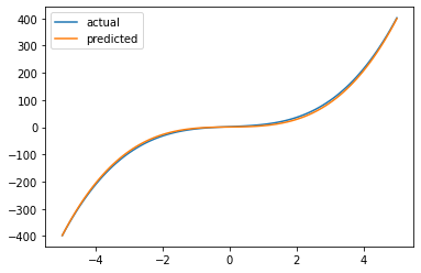
We see that the predicted weights are quite far off from the actual values, but plotting the graph of the two lines in fact show us very similar lines. The reason why the converged result is so different is due to the loss function having many minima, thus we would arrive at a different solution depending on where we initialised our weights and bias.
For the logistic example, we need to define our sigmoid function in order to work out the gradients, and to correctly backprop. them. Skipping the derivation of the derivative of the sigmoid, we have the following:
\begin{equation}
\sigma(x) = \frac{1}{1 +e^{-x}}
\sigma’(x) = \sigma(x)(1 - \sigma(x))
\end{equation}
def _sigmoid(x): # dummy sigmoid, doesn't calculate the gradient
    return 1 / (1 + np.exp(-x))

def sigmoid(input):
    x = input.num
    z = _sigmoid(x)
    y = Scalar(z)
    dy_dx = z * (1 - z)
    input.grad += dy_dx
    y.creators = [input]
    return y


def LogReg_data(b, w1, n = 20):
    x1 = np.linspace(-10, 10, n)
    X = []
    y = []
    for i in range(n):
        X.append([
                  Scalar(x1[i]),
                  ])
        z = b + (x1[i] * w1)
        target = _sigmoid(z)
        y.append(Scalar(target))

    return X, y


actual_b = 2
actual_w = 5
X, y = LogReg_data(actual_b, actual_w) # generate a data set with bias 2, w1 = 6 and w2 = 4

# the goal is to use grad descent to find approximations for b, w1, w2 close to their actual values
bias, w1 = Scalar(1), Scalar(1)# we initialise out model parameters to 0

for i in range(20): # we train for 10 epochs
    for j in range(len(X)): # loop through each datapoint
        x1 = X[j][0]
        target = y[j]
        y_hat = sigmoid(bias + (w1 * x1)) # prediction with the current weight
        loss = square(target - y_hat) # calculate the loss with the squar eloss function
        loss.grad = 1 # reset the loss gradient
        loss.backward() # backpropagate the gradients, starting from loss
        # take a step towards minimum
        bias.num -= 0.001 * bias.grad
        w1.num -= 0.001 * w1.grad
        # reset everything
        bias.grad = 0
        w1.grad = 0

        x1.grad = 0
        target.grad = 0
print("1. Linear Regression: y = 2 + wx + eps")
print(f"predicted bias: {bias.num:.2f}, predicte weight: {w1.num:.2f}")
print(f"actual bias: {actual_b}, actual weight: {actual_w}")

x = np.linspace(-10, 10, 100)
y1 = _sigmoid(2 + (5 * x))
y2 = _sigmoid(bias.num + (w1.num * x))
print(f"Loss: {((y1 - y2)**2).mean()}")
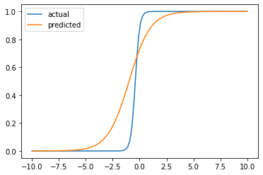
1. Linear Regression: y = 2 + wx + eps
predicted bias: 0.99, predicte weight: 1.01
actual bias: 2, actual weight: 5
Loss: 0.014717625247181693
plt.plot(x, y1, label = "actual")
plt.plot(x, y2, label = "predicted")
plt.legend()
<matplotlib.legend.Legend at 0x7fda09621090>
Final Words
I think this post has gone on for long enough so I will stop here. I hope my explanation on backprop. has been helpful, however, as I am still figuring things out it is very likely that I have made a mistake somewhere and I would appreciate if you would point it out to me by email.
Next Part
As you can see from the machine learning experiments above, the code we have to write just to train a simple model is rather… ugly. The next part will see us cleaning up some of the code by adpating a vectorised operation on our custom “Scalar” class, and we will create a better template to better organize our code.